Computing and visualizing descriptive statistics
Here we use the powerful descriptive and visualization tools offered by TraMineR to gain knowledge from the
mvad data set. Single commands compute transversal or longitudinal descriptive statistics and display them in nice looking plots. The commands used to generate the plots are given
below the Figure.
- Create a state sequence object from the mvad data set.
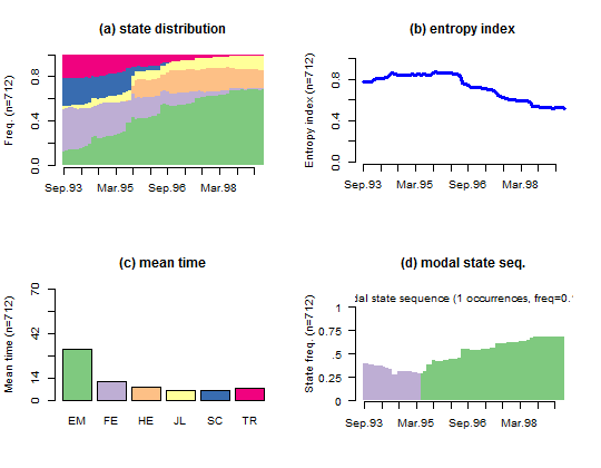
- Divide the graphic area in 2 rows and 2 columns (we want to include four different plots in the same figure).
par(mfrow = c(2, 2))
-
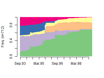
Compute and plot the state distributions by time points. Borders surrounding the bars are removed for nicer output. The display of the legend is deactivated since we include several plots in the same figure.
seqdplot(mvad.seq, with.legend = FALSE, border = NA)
-
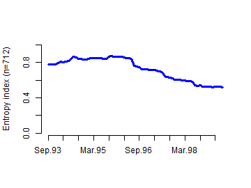
Compute and plot the transversal entropy index (sequence of entropies of the transversal state distributions).
seqHtplot(mvad.seq)
-
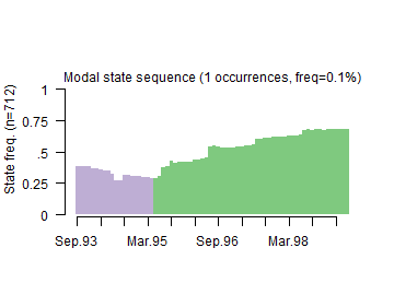
Plot the sequence of modal states of the transversal state distributions.
seqmsplot(mvad.seq, with.legend = FALSE, border = NA)
-
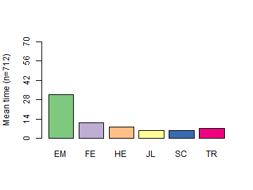
Plot the mean time spent in each state of the alphabet.
seqmtplot(mvad.seq, with.legend = FALSE)