Run discrepancy analyses to study how sequences are related to covariates
With TraMineR, it is very easy to analyze the discrepancy between sequences and visualize the results. Such analyses usefully highlight how the state sequences are related to one or more covariates (See
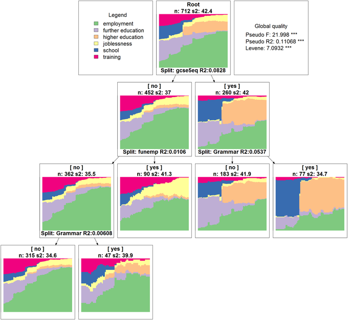
Studer et al., 2011). For instance, the figure below displays a regression tree for the state sequences grown from their pairwise distance matrix. It shows that, among the considered covariates,
gcse5eq explains the greatest part of the between-individual variability of the sequences. For youngsters with bad results at the end of compulsory school,
funemp is the most significant covariate. We can see that, among those with bad qualification at end of compulsory school, those who had an unemployed father have much more chance to experience joblessness. We give details about how to conduct the analysis and visualize the results
below the Figure.
- Create a state sequence object from the mvad data set.
-
Compute a distance matrix.
submat <- seqsubm(mvad.seq, method = "TRATE")
dist.om1 <- seqdist(mvad.seq, method = "OM", indel = 1, sm = submat)
-
Compute and test the share of discrepancy explained by the categorical gcse5eq covariate.
The gcse5eq covariate explains 8.3% of the discrepancy and the association is significant (p-value<0.001). The Levene statistic serves to test equality of the within-group discrepancies.
da <- dissassoc(dist.om1, group = mvad$gcse5eq, R = 5000)
print(da$stat)
| |
t0 |
p.value |
| Pseudo F | 64.058 | 2e-04 |
| Pseudo Fbf | 62.101 | 2e-04 |
| Pseudo R2 | 0.083 | 2e-04 |
| Bartlett | 1.311 | 2e-04 |
| Levene | 14.773 | 4e-04 |
|
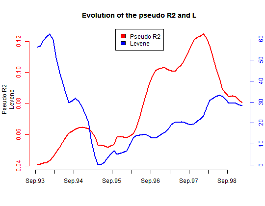
- Plot the evolution of the association between the state sequences and the gcse5eq covariate on six month sliding-windows. We observe that gcse5eq has a long term effect, since the pseudo R2 tends to increase alongside the time axis.
Gdiff <- seqdiff(mvad.seq, group = mvad$gcse5eq, cmprange = c(0,
    5), seqdist.args = list(method = "OM", indel = 1, sm = submat))
title <- "Evolution of the pseudo R2 and L"
plot(Gdiff, stat = c("Pseudo R2", "Levene"), lwd = 2, main = title)
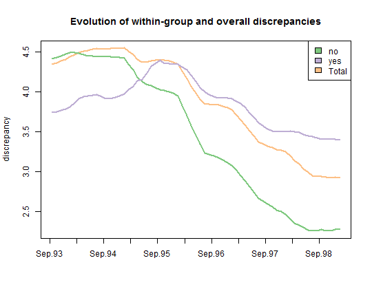
- Plot the evolution of the within-group discrepancy on six month sliding-windows.
title <- "Evolution of within-group and overall discrepancies"
plot(Gdiff, stat = c("discrepancy"), lwd = 2, main = title, legend.pos = "topright")
- Grow a regression tree for the state sequences and display the results. The graphical display uses GraphViz (Download GraphViz), which must be installed on your system for the function seqtreedisplay to work.
st <- seqtree(mvad.seq ~ gcse5eq + Grammar + funemp, data = mvad,
    R = 5000, diss = dist.om1, pval = 0.05)
seqtreedisplay(st, type = "d", border = NA)
--------------
Studer, M., Ritschard, G., Gabadinho, A. & Müller, N.S. (2011), Discrepancy analysis of state sequences. Sociological Methods and Research, 40(3), 471-510. Available here.